The Image gallery is a relatively new feature in our web application, providing a means of navigating our image library for a given location with folders and filters. After searching for a property, you can hit the ‘See all images at this location’ link in the infobox to bring it up. You can then browse all imagery we have at the location, filtering by year, image type, orientation and more.
The only downside is that if you click one of the thumbnails and go into full screen interactive mode, you have to repeat the entire process of filtering to then get to the next image you want to see.
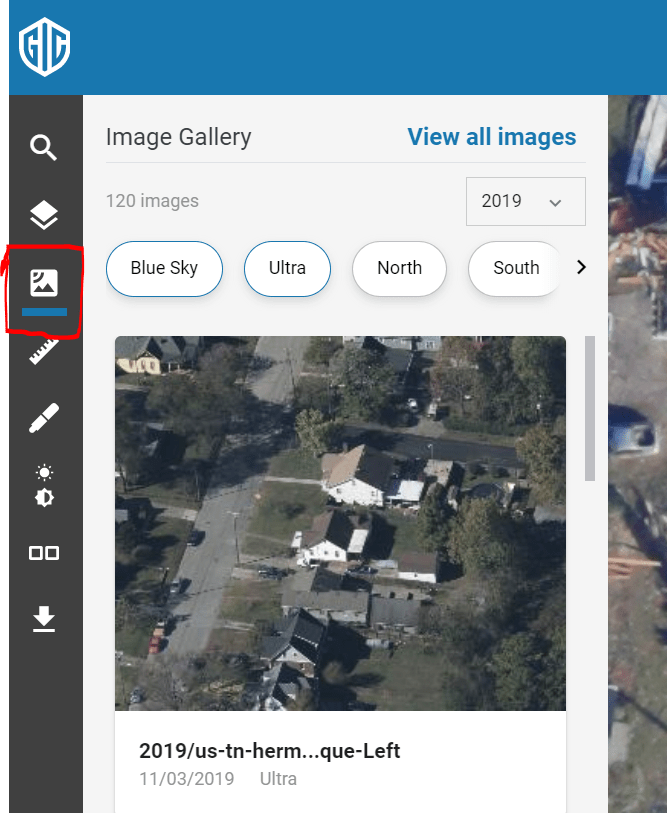
Well, things just got a lot more convenient in the Vexcel Web App! The new Image Gallery Sidebar stays docked in the left rail enabling you to quickly filter, view and repeat without losing context. It is the third tool down on the toolbar as highlighted here:
All of the same filters from the full screen interface are present. Choose your year, filter by image type or orientation, then click away on the preview thumbnails. As you click, each image will take over the interactive map window. You can navigate around in the interactive window, change orientation, etc… and then simply click the next thumbnail you want to interact with. this is the smoothest way to explore our image library to date, although I still love using the history tool on occasion.
A question came in to support this week on how to select the best image for each day of collection. When we fly and collect aerial imagery, we will typically end up with many shots of a property, each just a second or 2 apart. Add in the fact that we have multiple images in each oblique orientation of north, south, east and west and you can see how we have on the order of 50 views of each property every time we fly over. All of these images can be very helpful in doing detailed analysis of a property, but sometimes you want to present just the best image on each day of flight in your application.
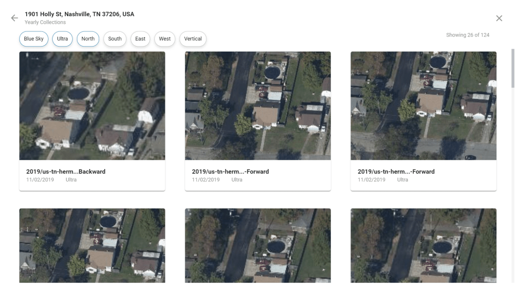
Here is an easy solution that takes advantage of the date filters on the ExtractImages endpoint. there are three steps in the process.
Query the catalog to get all of the metadata for all collections at your coordinate of interest
Parse the results to create a list of dates that have imagery
Make a follow up call to ExtractImages for EACH of the days found in step two and ask for the single best image on that day
Here is a sample app showing the three steps together. You need to plug in your Vexcel account credentials, then specify any lat/long coordinate and hit go! The app is all client-side JavaScript so just view source to see the API calls being made.
Using this coordinate (36.175216, -86.73649), lets look at the actual API calls for steps 1 and 3
Step 1. Find all Image metadata a the point
We’re going to focus on just the Nadir (vertical) imagery. Here is the API call to query the Vexcel catalog at this coordinate. in the response you’ll see we have 57 Nadir images for this property!
Step 2. Parse the Json from step one to find the dates with at least 1 image.
We want to build a list of days that have at least one image. The best way to do this is to sort the 57 images by capture date, then iterate through and build a list of unique dates. In this case we will end up with a list of 5 unique dates from September 9, 2012 to March 4, 2020
Step 3. Request the best image on each date found in step 2
For each of these calls, note the initDate and EndDate parameters. Also, note the mode=one which will return the best image in the date range. We can make a call to ExtractImages like this for each of the 5 dates we found in step 2. Here are a couple of them with their resulting image.
This video tutorial shows how to use the Vexcel API and Azure’s Custom Vision service to find damage after a fire or wind catastrophe across an arbitrary area. You can download the app from the previous post where we looked at how to analyze specific properties coming from a CSV file. The big difference here is that you don’t need a list of properties to analyze. instead you set the corners of a bounding box, and all of the properties within the box are analyzed. Microsoft’s building footprint files are used to find the candidate properties to test. In the image above, the white pins represent ALL of the building structures in the tested region. Each was run through the damage model with the structures determined to be destroyed showing as red pins.
Try it out and send your feedback along. you will need to have a Vexcel API account in order to run the app.
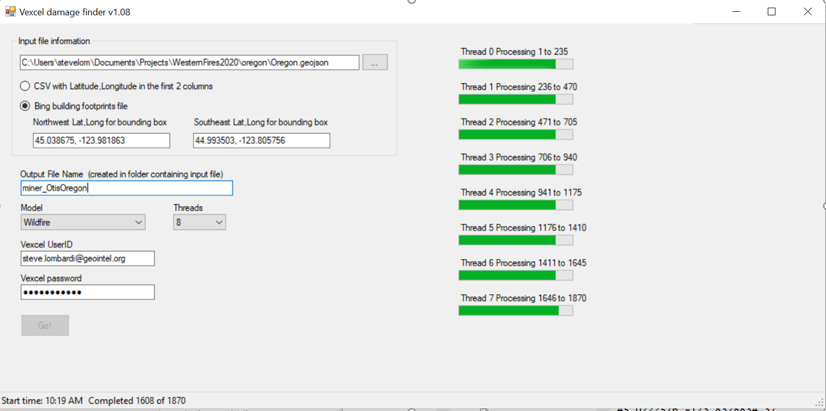
Over the last weeks, I shared a three part tutorial on training a model to identify homes damaged by wildfire, hurricane or tornado using Azure Cognitive services. In the final part we looked at how to use the Cognitive Services API to automate analysis of properties. Building on that, I’ve used the API to create an app to read a CSV file of coordinates, request the imagery from Vexcel API, and run each through the Cognitive services model. the results are written out to a CSV file that you can then do further analysis with, as well as a KML file to load into a GIS. You will need your Vexcel Platform account credentials to run the app.
You can download a zip file containing the app (runs on Any flavor of Windows) and a couple of sample CSV files to run through it. Unzip everything to a folder and launch the .exe to get started.
Choose Your Input File Use the … button to browse and select your input CSV. The first column should contain latitude and the second column, longitude. Additional fields can follow. A couple of sample files are included in the zip that you can use as a template. (I’ll cover the building footprints option in the next article.)
Set a name for your output file a CSV and KML file will be created in the same folder as your input file. Specify a name for the root of the file. The appropriate extensions will be appended on.
Choose the appropriate model and processing threads there are two choices for model; Wildfire and Wind Damage. choose the one appropriate for the type of damage you are analyzing. You can choose from 1 to 8 processing threads.
Finally enter your Vexcel Platform credentials and hit the Go! button to get things started.
While the app is running, have a look in the output folder. You’ll see some temporary files being created there of the form OutputFilename_thread#. To prevent IO conflict, each thread writes to it’s own files and when the run is finished, these files will be appended together to form your final output KML and CSV files. You can then delete these temp files if you wish.
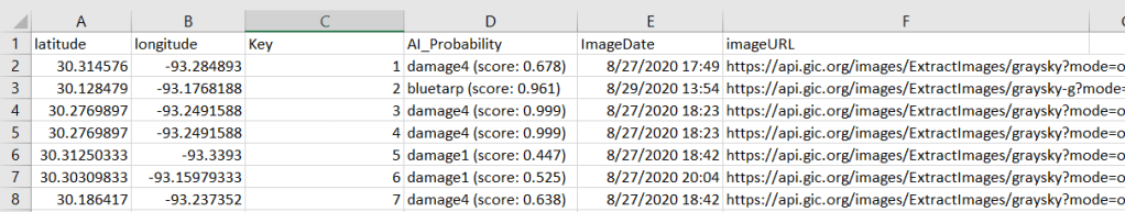
After processing is complete, open up the .CSV file in Excel or a text editor. You’ll see three fields have been appended to your input file representing the prediction from the model, the date of the image used in the analysis and a link to the image itself. In the screenshot below you can see this in columns D, E, and F respectively. If you were running the wind damage model, the predictions will go from Damage0 (no visible damage) to Damage4 (complete loss). The score shown is the probability the prediction is correct. For Wildfire, there are just 2 possible tags; Fire0 (undamaged) and fire2 (burned).
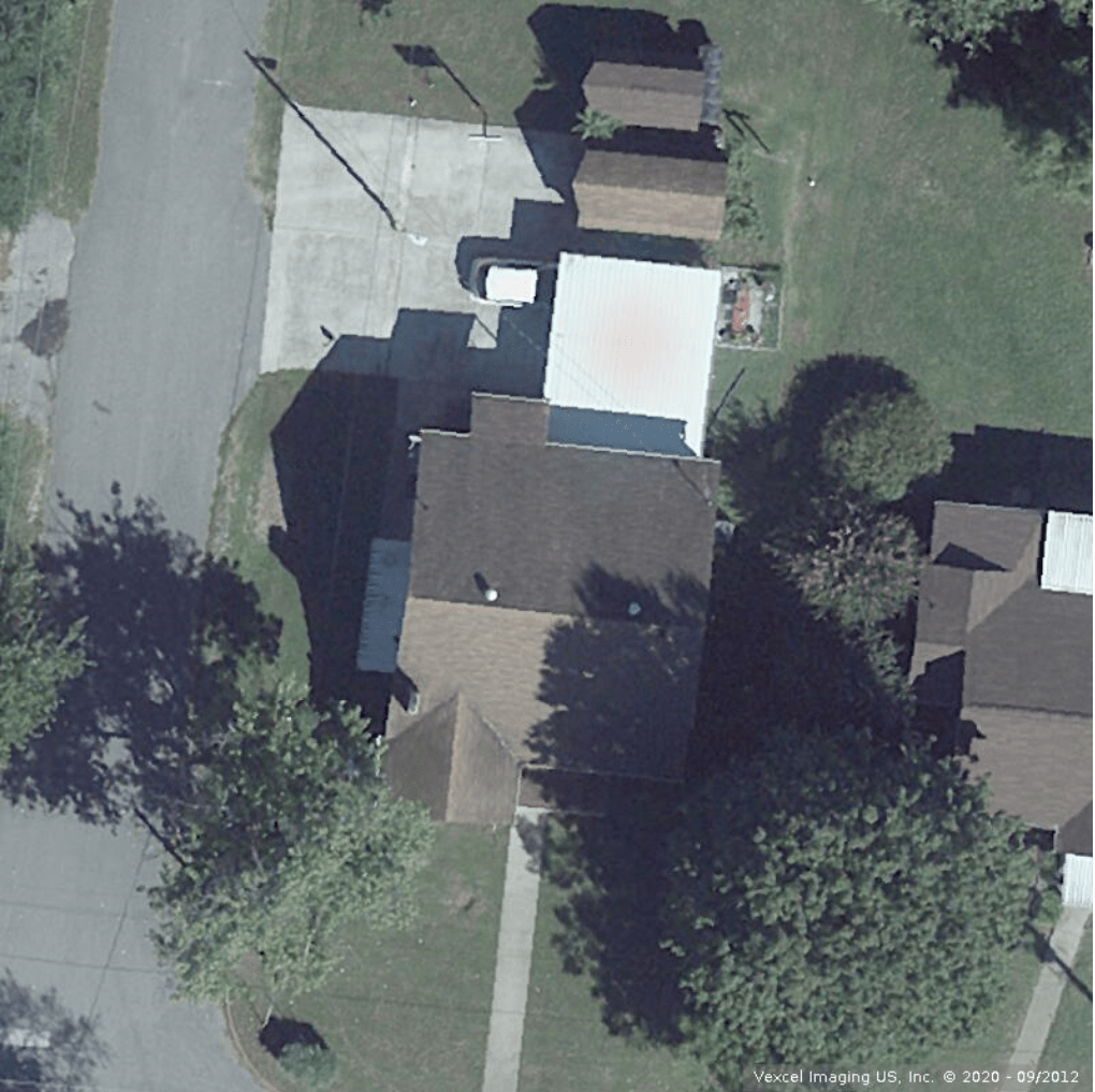
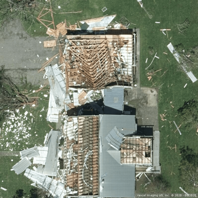
Let’s look at row 4, which scored Damage4 with very high probability. the ImageURL in Column F returns this image:
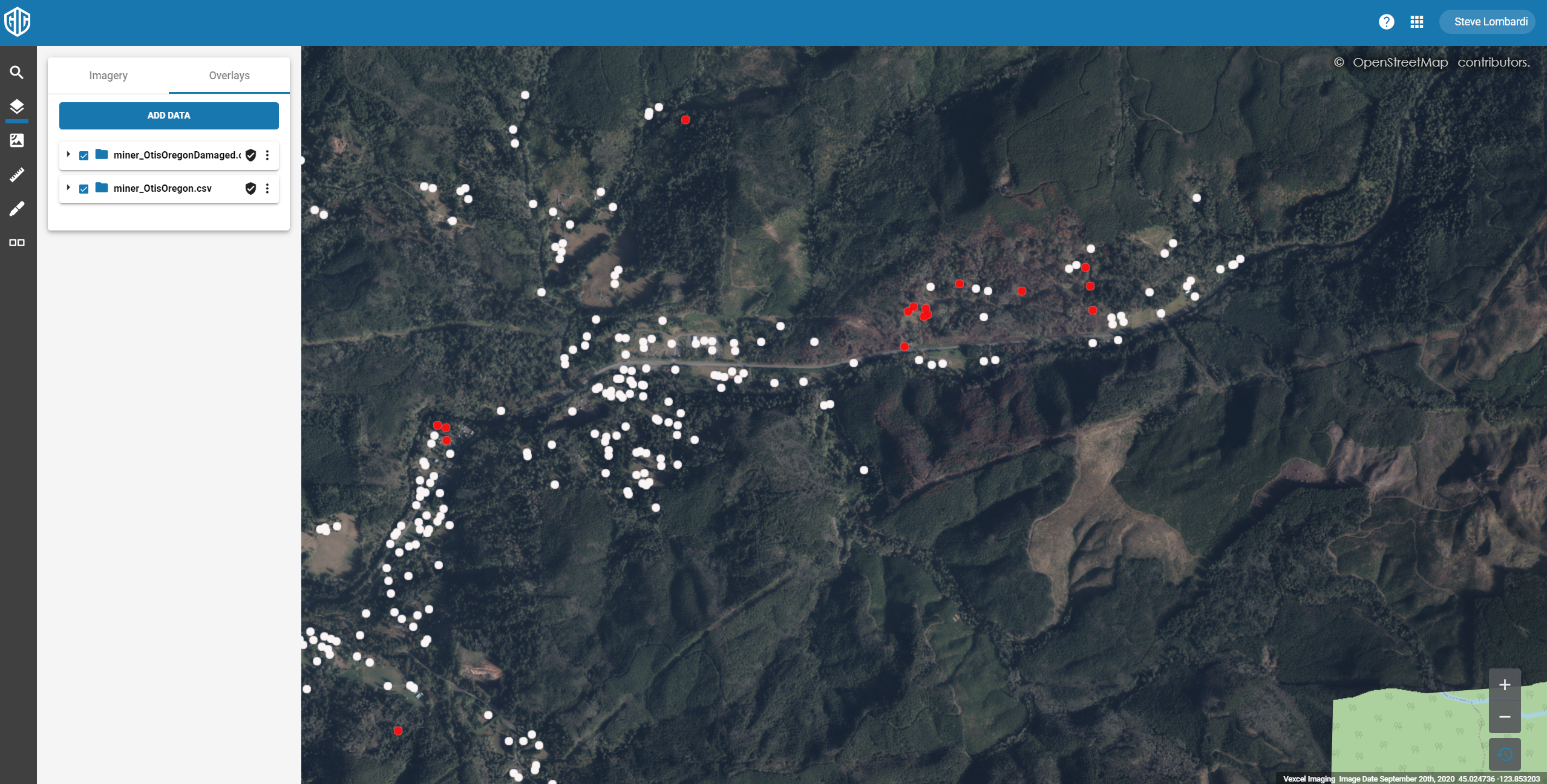
You can load the CSV or KML file into just about any mapping application which will certainly have support for either CSV or KML files. Lets use the Vexcel viewer to visualize a file of Fire Damaged properties in Otis Oregon. After the run was complete, I loaded the CSV file into Excel, sorted by the AI_Probability column, then cut all of the damage2 records into 1 file, and damage0 into another. this allows me to load them as two sperate layers in the Vexcel viewer.
In this first image you can see all of the properties in the region that were run through the app.
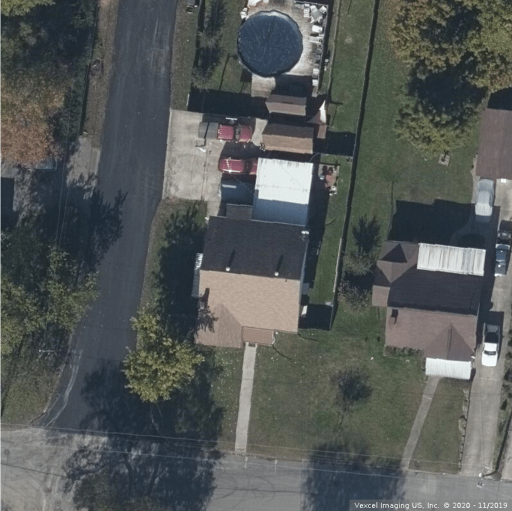
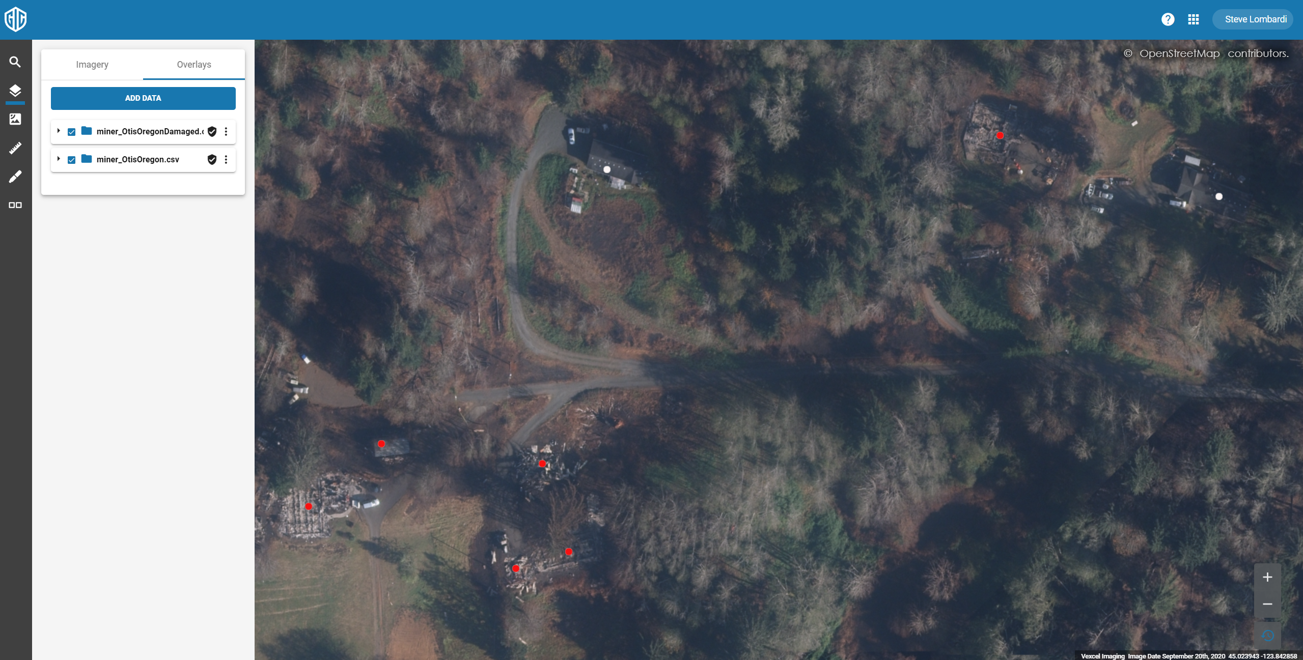
And in these next two, you can see the properties tagged Damage2 in red.
and here zoomed in to the damaged cluster in the northeast
KNOWN APP ISSUES
After appending the individual KML file there is a stray character on the last line of the file that prevents it from loading in some client apps. if you encounter this, load the file in a text editor and delete the last line with the odd control character. I’ll fix this as soon as I figure out what’s causing it 🙂
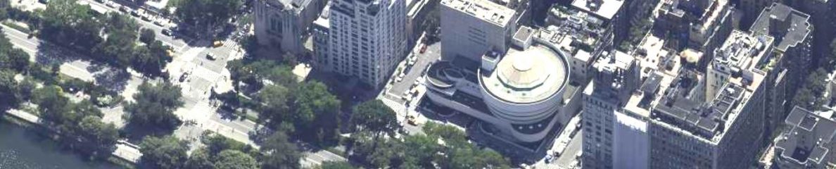
Among the data products we provide, Infrared imagery is among the more specialized. To help us understand what infrared imagery is and how we can best utilize it, I called on Bernhard Schachinger in our Graz office to share his insights. Bernhard is not only an expert in our camera systems, but also the processing of the raw data that comes from the sensor and the creation of our data products.
The image above is a high resolution example from Graz, where red shows clearly the vegetation, yellow a particular type of roof and almost normal greyish color tones show roads and other types of roof. In combination with RGB, this is a very important source of information for powerful image classification.
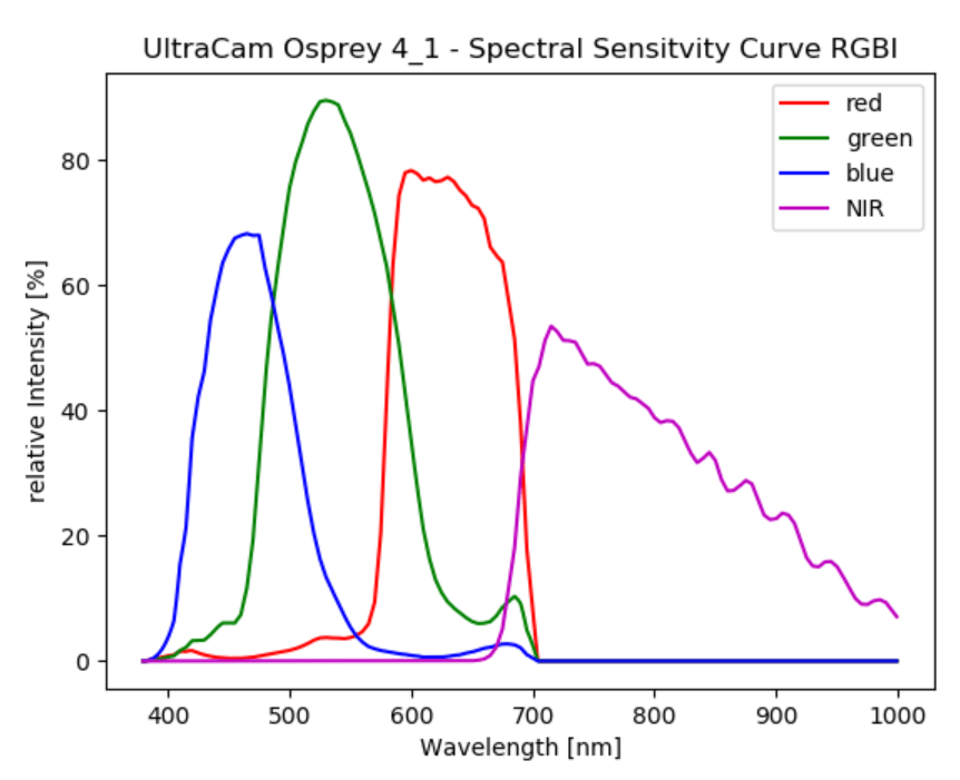
The near-infrared band (NIR) is close to the visible range of the red channel and covers the wavelength from ~670 nm to ~1050 nm. See the graph below for the spectral sensitivity curves for RGBI channels, as we include it in the camera calibration reports for Ultracam Osprey 4.1 (UCO 4.1).
The motivation to capture NIR is a characteristic of vegetation which is measurable in the reflectance. A good explanation can be found here on wikipedia. NIR can not only give some information about the type but also about the health/growing period of the vegetation.
Here is an important except:
Red edge refers to the region of rapid change in reflectance of vegetation in the near infrared range of the electromagnetic spectrum. Chlorophyll contained in vegetation absorbs most of the light in the visible part of the spectrum but becomes almost transparent at wavelengths greater than 700 nm. The cellular structure of the vegetation then causes this infrared light to be reflected because each cell acts something like an elementary corner reflector.
The phenomenon accounts for the brightness of foliage in infrared photography and is extensively utilized in the form of so-called vegetation indices (e.g. Normalized difference vegetation index). It is used in remote sensing to monitor plant activity
Color-infrared images (CIR) are created with this combination of bands: R = NIR, G = Red, B = Green. CIR imagery is mainly used for detecting vegetation and water bodies, but also supports the identification of roads and buildings. Examples for use cases:
To analyze the biomass, e.g. identification of forest areas with bad health for forestry or risk assessment (fires, bark beetle)
Analysis of agricultural fields, e.g. checking the growth rate, irrigation, use of fertilizers
Supporting classification tasks (vegetated, non-vegetated, water bodies)
Checking for living/dead vegetation after disasters
A useful tool to accomplish these tasks is the Normalized difference vegetation index (NDVI), which can be calculated from our imagery. here is a good article explaining NDVI in detail. The advantage of the NDVI vs RGB-based methods is that this index compensates for changes in light conditions, surface slope, exposure and such external factors.
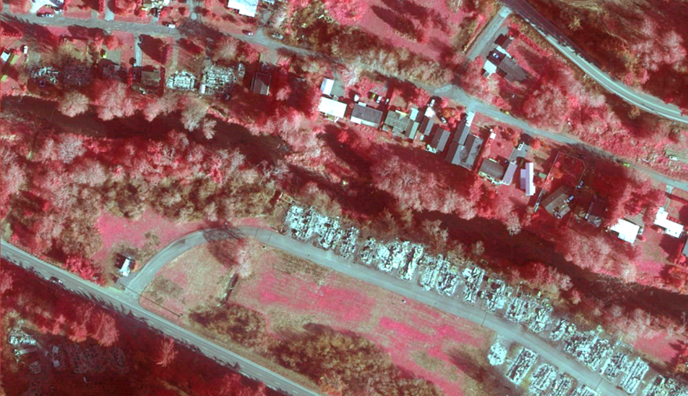
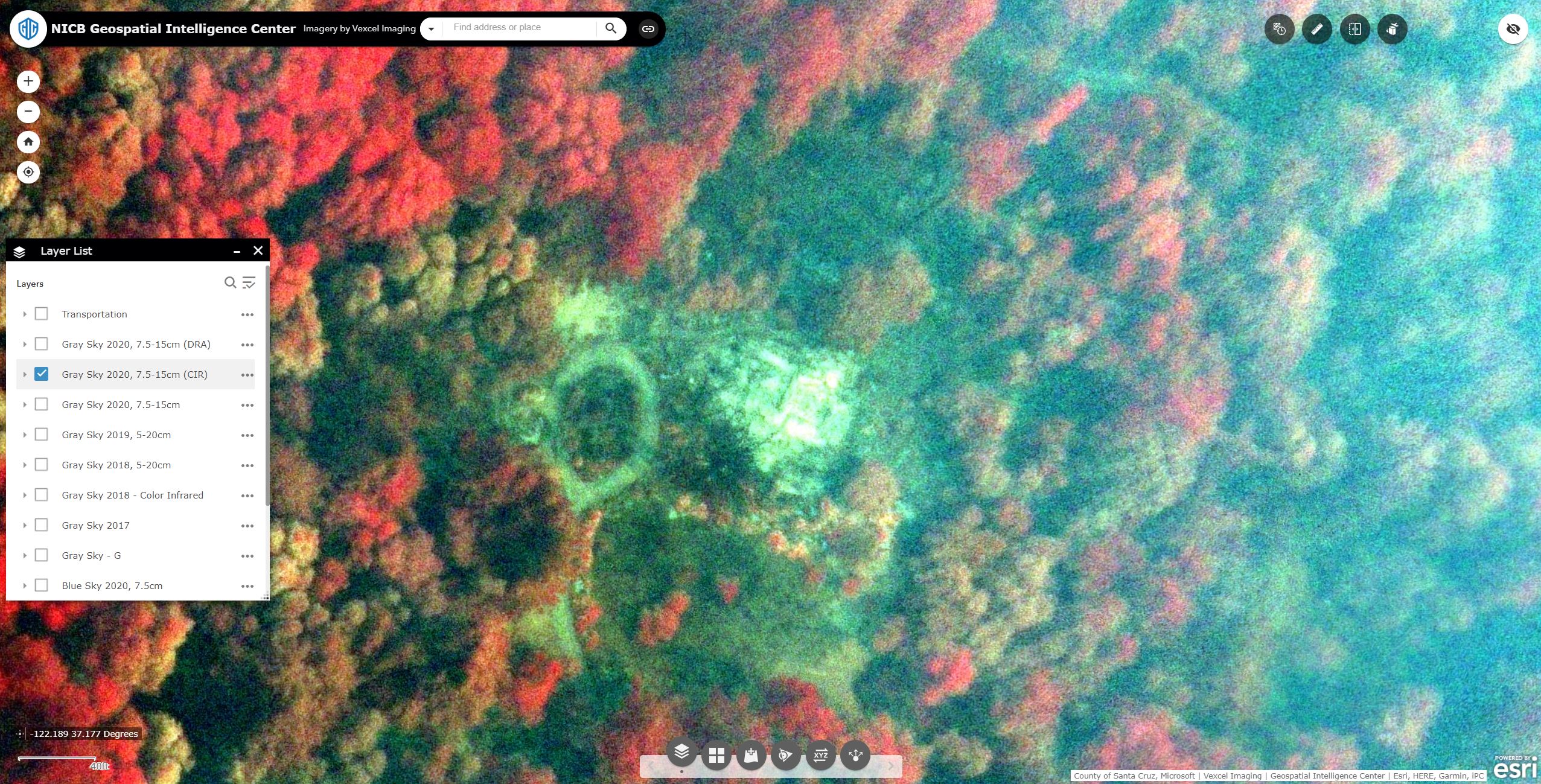
Here is another example from our disaster response imagery pulled from the recent Oregon wildfires. we can see with red color healthy trees/grass and with brownish/greyish color tones burnt vegetation. Buildings are also clearly visible. In this case, the CIR is an additional help for the human eye to identify burnt areas.
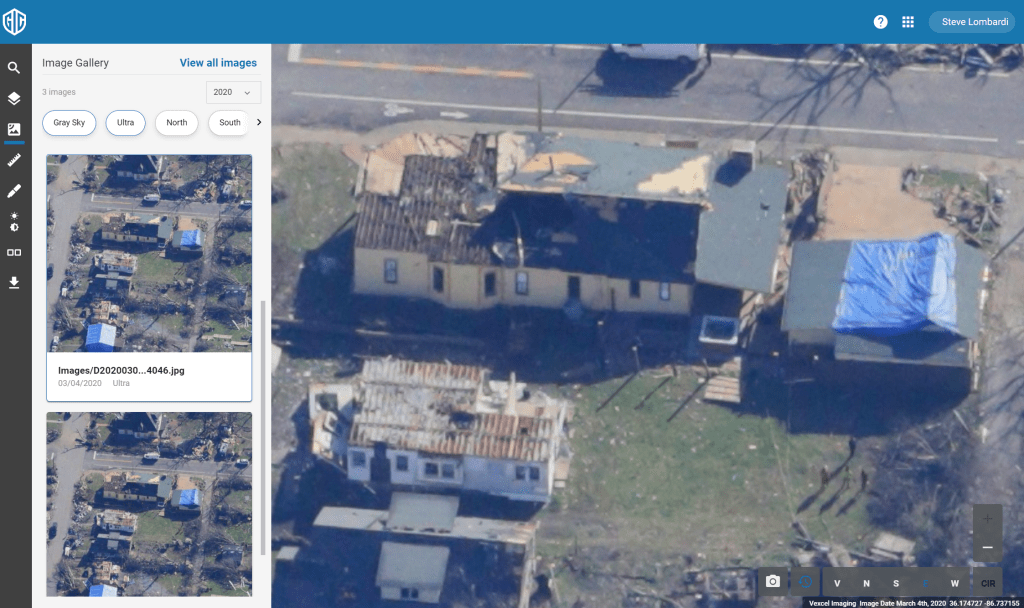
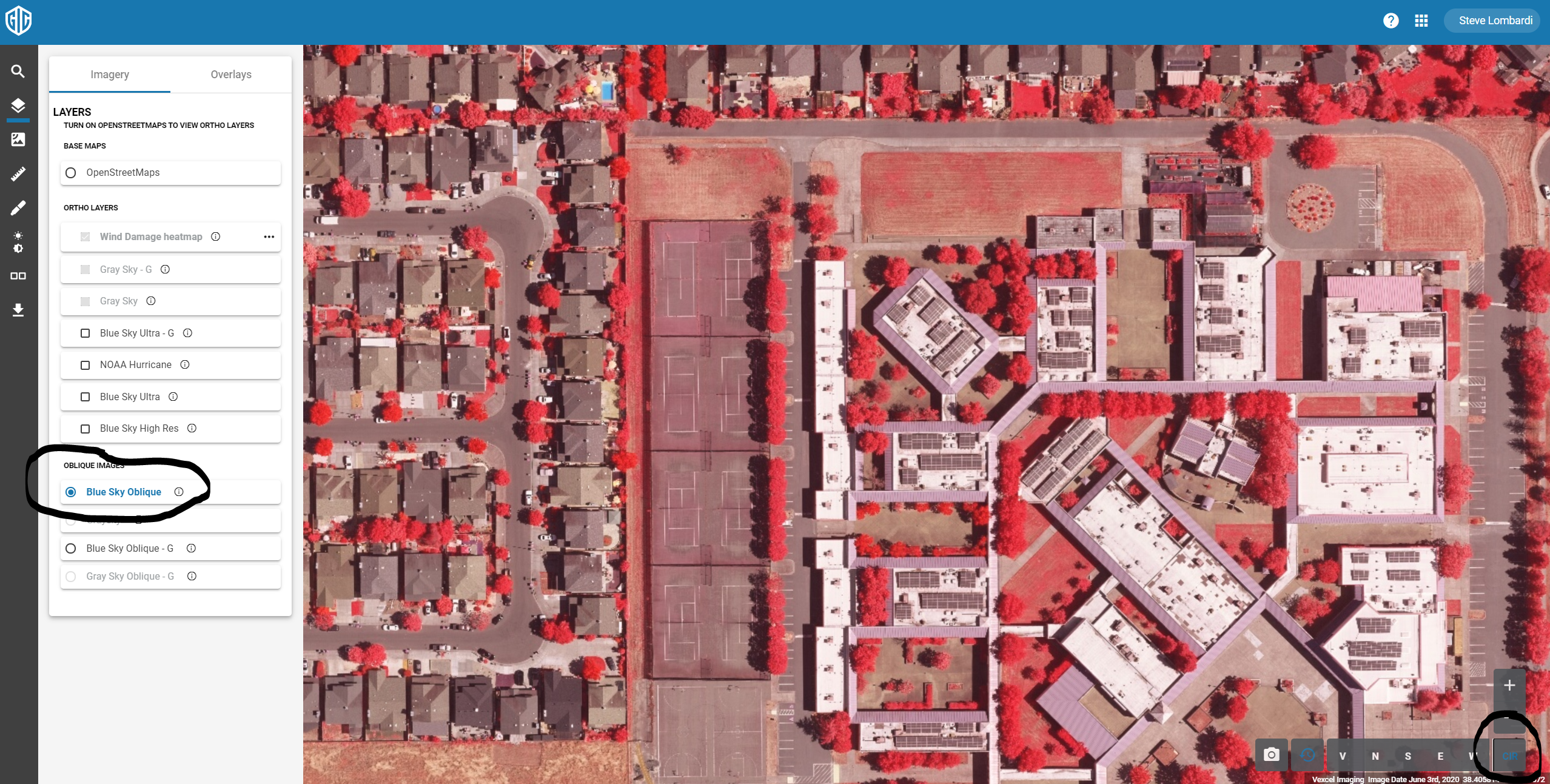
CIR imagery has been available via our API’s for a while now, but this week we introduced this image type into our web application. To access it, go to Oblique mode for the Blue Sky Ultra layer and click the CIR button in the lower right of the screen as shown here:
Finally! In the first 2 parts of this tutorial series we focused on training models on Azure’s Custom Vision platform to perform recognition on Vexcel imagery. But now the best part; We’ll use the REST API exposed by Custom Vision to handle the repetitive task of running multiple properties through the model. This opens up use cases like analyzing a bunch of property records after a tornado or wildfire using Vexcel graysky imagery. Or checking to see which homes have a swimming pool using Vexcel Blue sky imagery.
In this tutorial we’ll use c# to call the Vexcel API and Custom Vision API, but you should be able to adapt this to any language or environment of your choosing. The application will make a call to the Vexcel platform to get an auth token, subsequent calls to generate an ortho image of a given property, then pass that image to our model on Custom Vision for recognition. Once you have this working, its easy to take it to the next step to open a CSV file containing a list of locations, and perform these steps for each record..
Step 1: Publish your model
In the previous tutorials we trained a model to recognize objects or damage in aerial imagery. We can now make programmatic calls to the model using the Custom Vision API, but first we need to publish the trained iteration, making it accessible by the API.
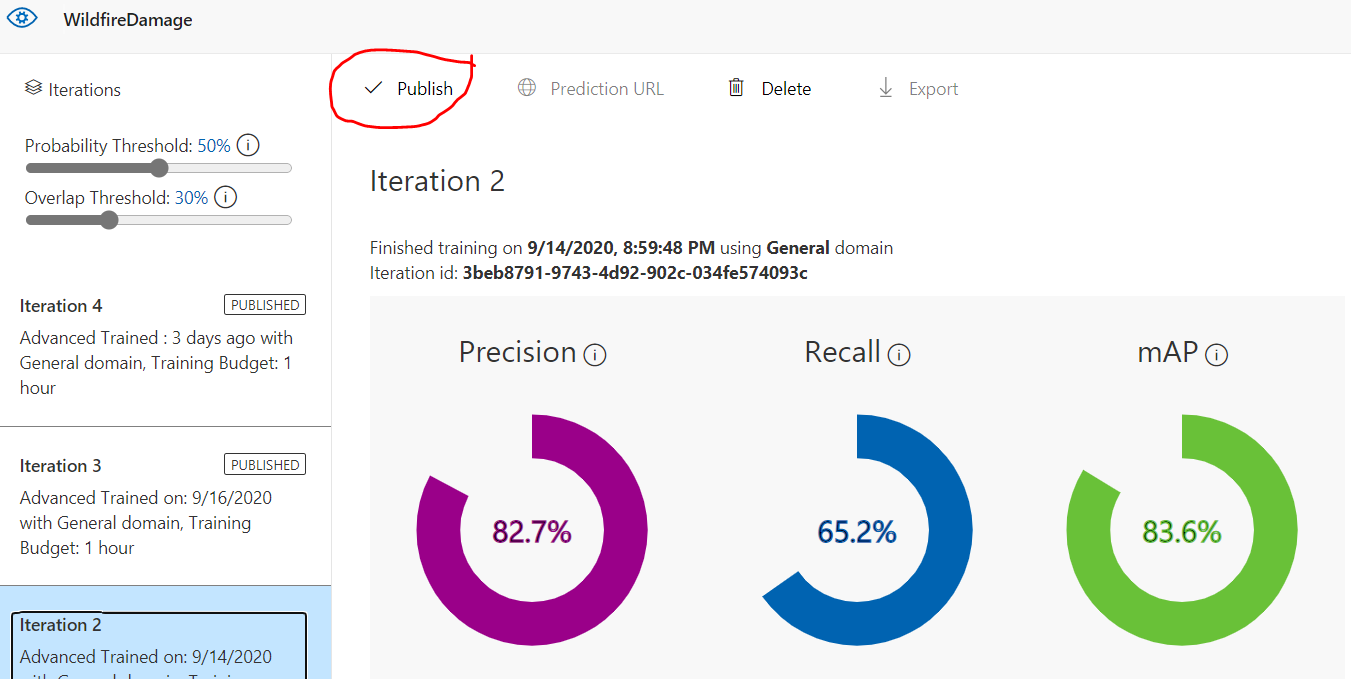
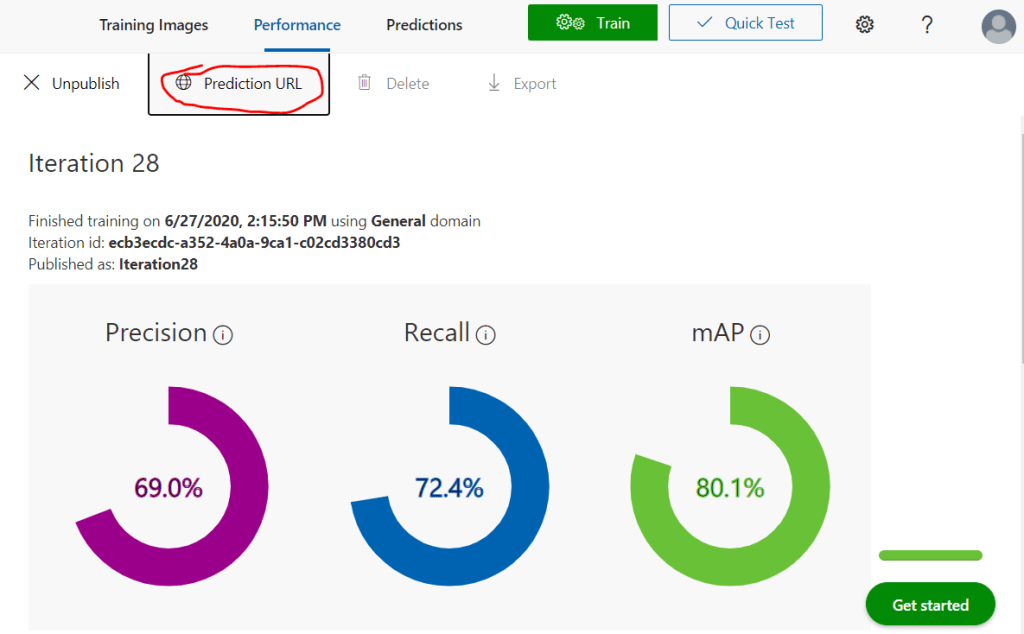
This is easy to do. In the Custom vision Dashboard, go to the Performance tab, select your iteration, and hit the ‘publish’ button as highlighted here.
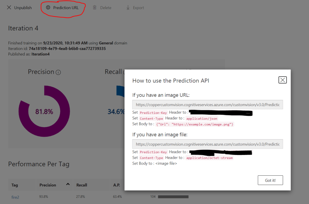
Once the publish is complete, the ‘Prediction URL’ link will become active. Click it to view the parameters for your model that you will need when making calls with the API. The ‘Iteration ID’ is shown on the main dashboard page. The prediction key is visible in the dialog that pops up, as well as the REST URL which will contain the project ID. Take note of all of these values. We’ll use them in a moment.
Step 2: Generate an Authentication token with the Vexcel API
Each API call to the Vexcel platform requires and auth token to be passed. When your app starts up, you can call the login service to generate one and use it for all subsequent calls. An auth token is good for up to 12 hours.
The fetchURL() method is used to make an HTTP request and return the response as a string. Here is a simple implementation for C#.
string html = "";
try
{
    WebRequest request = WebRequest.Create(url);
    WebResponse response = request.GetResponse();
    Stream data = response.GetResponseStream();

    using (StreamReader sr = new StreamReader(data))
    {
        html = sr.ReadToEnd();
    }
}
catch (Exception ex)
{
     //handle the error here
}
return html;
Step 3: Generate a URL to request an image of a property
There’s generally two steps to request an image from the Vexcel library; first query the catalog to see what is available, then request the appropriate image. Lets do exactly that for this coordinate damaged in the Oregon wild fires recently: 45.014910, -123.93089
We’ll start with a call to FindImages(). This service will return a JSON response telling us about the best image that matches our query parameters. Those parameters include the coordinate, a list of layers to query against, and the orientation of the image we want returned. For the layer list we are passing in Vexcel’s two gray sky layers; we want the best (most recent) image across any catastrophe response layer. We’ll set orientation to Nadir as we want a traditional vertical image, but you can also query for Vexcel’s oblique imagery with this parameter.
In the Json response, we’ll have all of the information we need to request a snippet of imagery with the ExtractImages() method. This workhorse provides you access to all of the pixels that make up the Vexcel library, one snippet at a time carved up to your exact specification. As you can see below in the code, the first bit of metadata that we’ll grab is the date the image was taken. This is one of the most important pieces of metadata regardless of what kind of application you are building; you’ll always want to know the date of the image being used. And then most importantly, we’ll form a URL to the ExtractImages endpoint with all of the parameters needed to get the image we need, as provided by the FindImage() call above.
Step 4: Pass the image to Custom vision for analysis
Its finally time to pass the Image snippet to Custom Vision for recognition. You’ll need the details from step 1 above where you published your model. You can return to the Custom Vision dashboard to get them. Here is the c# to make the API call and get back a JSON response indicating what tags were found in the image.
The last bit of code is to parse the returned JSON to find the tags discovered in the image. Keep in mind that there can be multiple tags each with their own probability score returned. We’ll keep it simple and loop through each tag looking for the highest probability, but in your implementation you could choose to be more precise than this, perhaps by considering the position of each discovered tag relative to the center of the image.
That’s it! Now that you can programmatically analyze a single image, its a small step to put a loop together to step through a large table of properties. In a future tutorial here on the Groundtruth, we’ll do something similar building on the code above to create a highly useful application.
In Part One of this three part tutorial, we trained a model using Azure’s Custom Vision platform to identify Solar Panels on rooftops using Vexcel’s Blue sky imagery. Here in part two we are going to work with disaster response imagery (aka graysky imagery) to identify buildings damaged in Wildfires.
The main difference here is that we will train the model on two tags, one representing buildings that have not been burned, and a second tag representing buildings that have been destroyed in the fire. Other than that, the steps are identical to what we did in Part One.
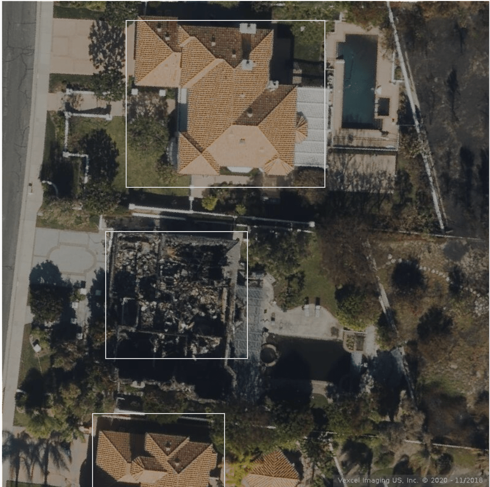
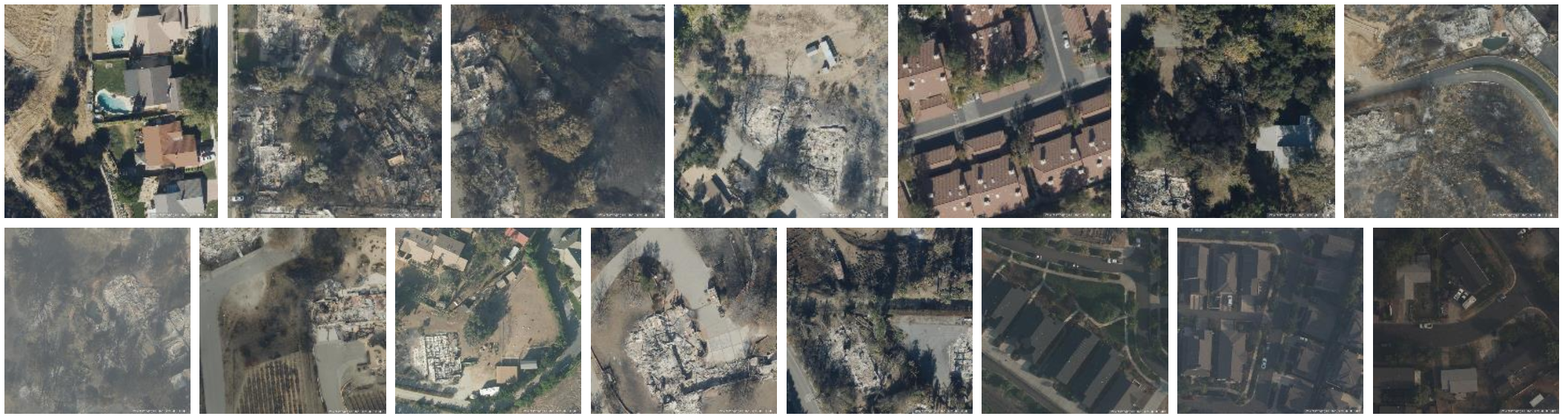
In this image you can see a good example of both tags that we will be training.
Step 1: Create a Custom Vision Account
If you completed part one of the tutorial, you’ve already setup your Custom Vision account and can proceed to step two below. But if you have not set up you Custom Vision account yet, Go back to part 1 of the previous tutorial to complete step 1 (account setup) then return here.
Step 2: Collect a bunch of images for tagging
You’ll need to have 15 or more images of buildings NOT damaged by fire and 15 showing damaged buildings. Its important that both sets of images are pulled from the graysky data.
Create a folder on your local PC to save these images too. There are several ways you can create your images. One easy way is to use the GIC web application, browse the library in areas where there is wildfire imagery, then take a screen grab and save it to your new folder. Here are some coordinates to search for that will take you to areas with good wildfire coverage:
42.272824, -122.813898 Medford/Phoenix Oregon fires 47.227105, -117.471557 Malden, Washington fires
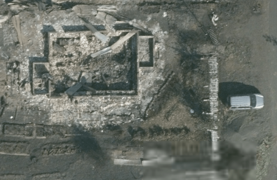
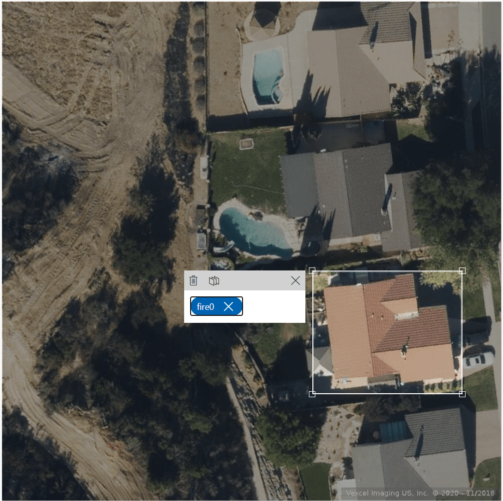
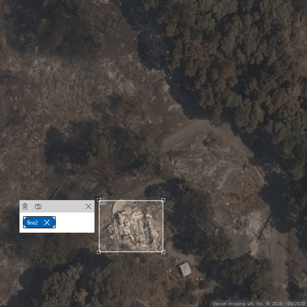
Here are two good representative images similar to what you are looking for. First an example of a destroyed building
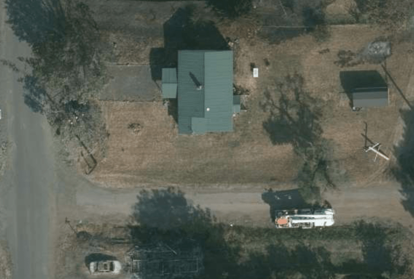
and an example of a structure still standing after the fire:
When you have 15 or more good examples of each in your folder, move on to the next step. Its time to tag our images!
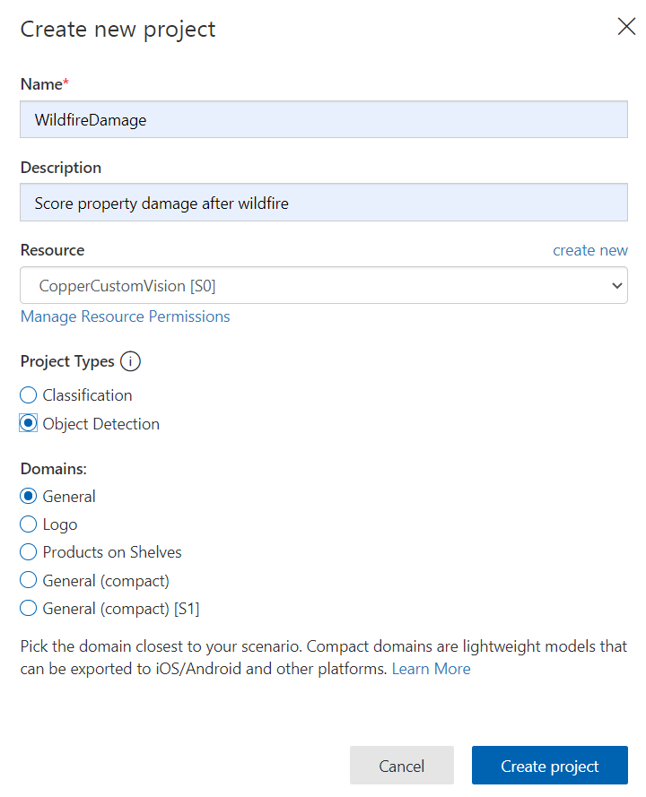
Step 3: Create a new project in your Custom vision account
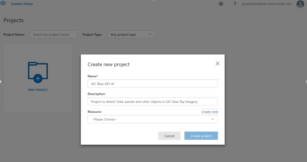
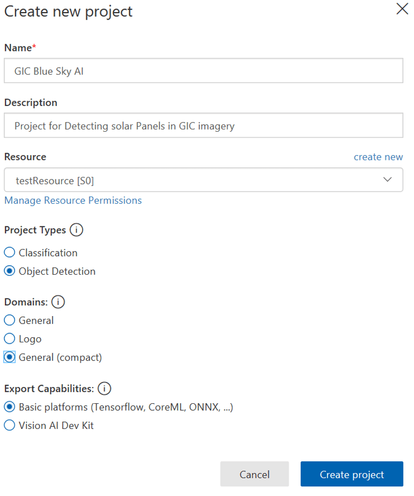
Click the ‘New project’ button and fill in the form like this:
If this is your first project you’ll need to hit the ‘create new’ link for the Resource section. Otherwise you can select an existing Resource. Hit the ‘Create project’ button to complete the creation process. You now have a new empty project. In the next step we’ll import the images we created previously and tag them.
Step 4: Upload and Tag these images.
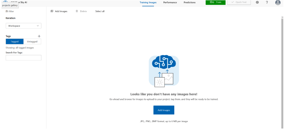
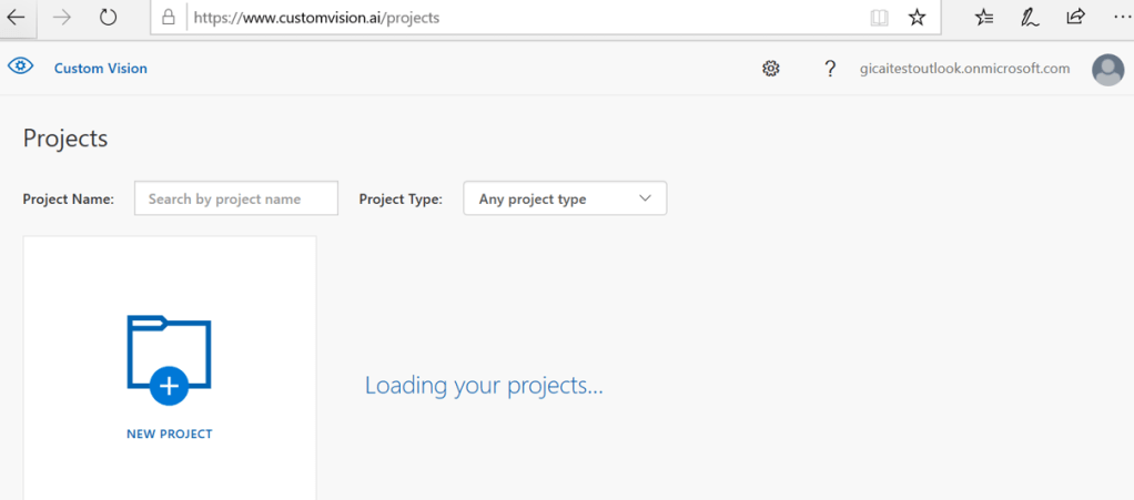
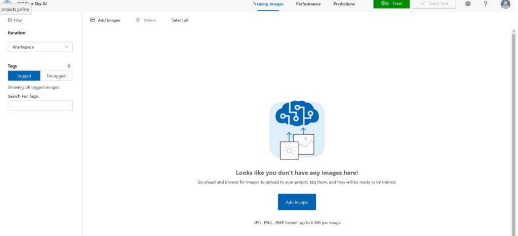
Your new empty project should look something like this:
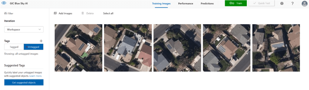
Hit the ‘Add Images’ button and import all of the images you saved earlier. You should see all of your untagged images in the interface like this:
Click on the first image of an undamaged property to begin the tagging process. Drag a box around the building structure. Its OK to leave a little buffer, but try to be as tight as possible to the building footprint. Enter a new tag name like ‘firenotdamaged’ And hit enter. If your image contains more than one structure, you can tag more than one per image.
Next choose an image with a building destroyed by fire and tag it in the same manner giving it a descriptive tag name like ‘firedamaged’.
Continue to click through all of your images and tag them. Some images might have a mix of burned and not burned structures. That’s OK, just tag them all appropriately.
Step 5: Train the model
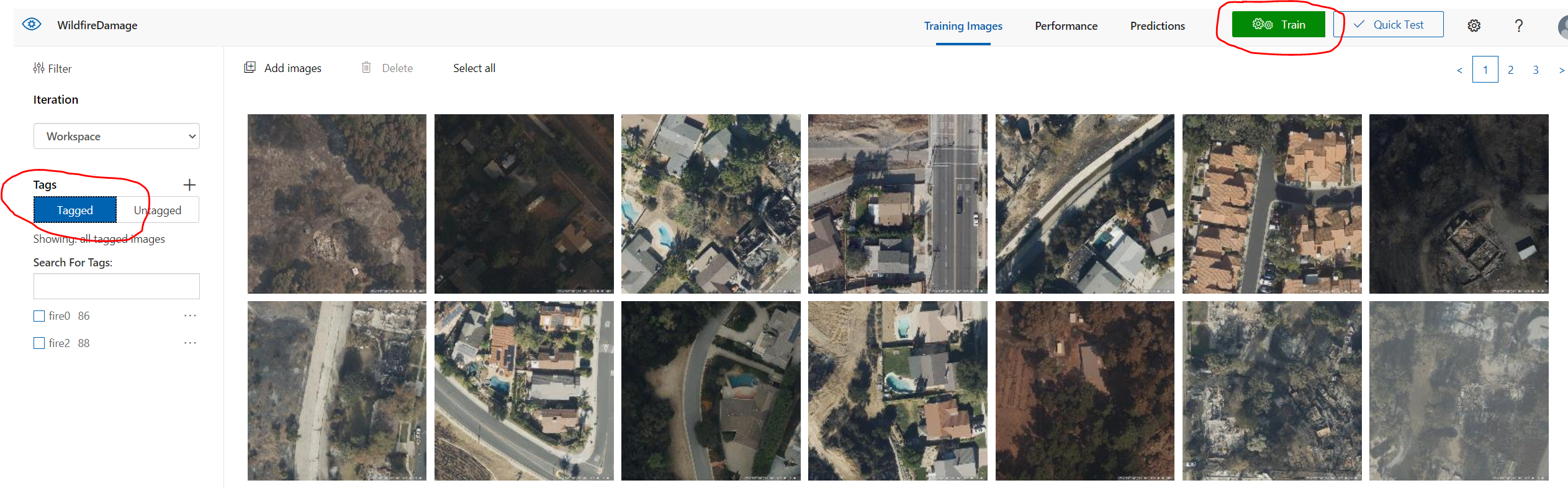
If you click the ‘tagged’ button as highlighted below, you will see all the images you have tagged. You can click on any of them to edit the tags if needed. But if you are happy with your tags, its time to train your model!
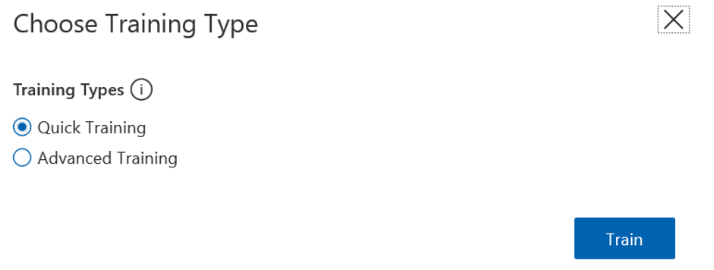
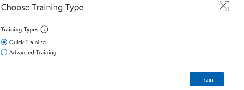
Hit the ‘Train’ button and select ‘quick training’ as your training type. Hit the ‘Train’ button to then kick off the training process. This will take around 5 minutes to complete, depending on how many images you have tagged.
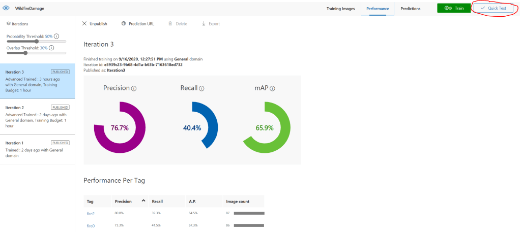
Step 6: Test the model
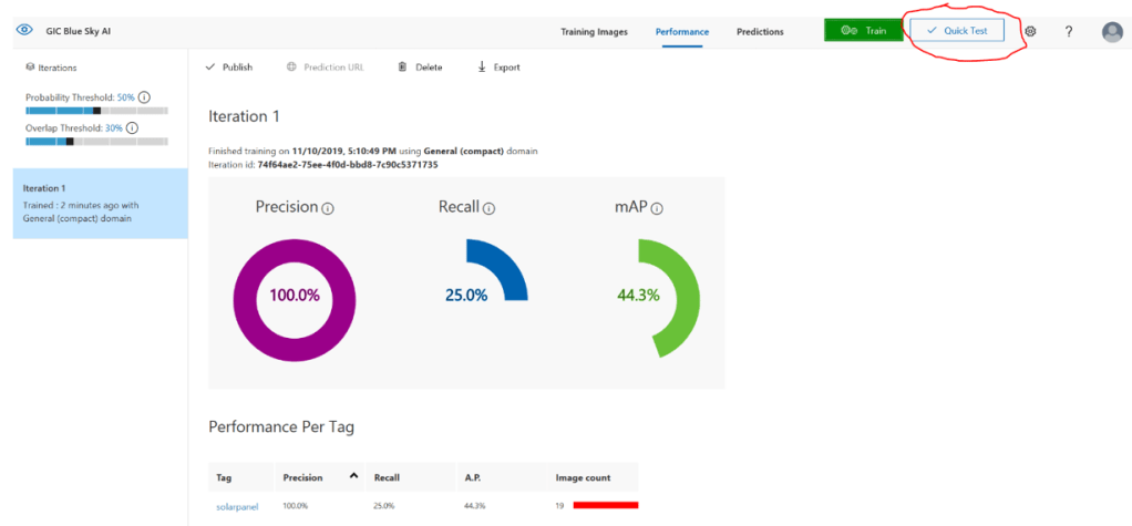
When training completes, your screen will look something like this:
Its time to test your model! The easiest way to do so is with the ‘quick test’ button as highlighted above. Using one of the techniques used in step 2 to gather your images, go and grab a couple more and save them to the same folder. Grab a mix of buildings, some destroyed and some not.
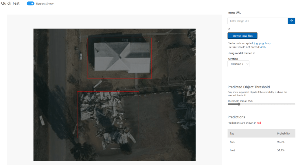
Hit the ‘Quick test’ link, and browse to select one of your new images. Here I selected an image that contained two adjacent structures, one destroyed and one not. You can see that both were correctly identified, although the probability on the burned building is a little low. this can be improved with tagging more images and retraining the model.
In Part three of this tutorial, we’ll use the API exposed by the Custom Vision Platform to build an app that can iterate through a list of properties and score each one
At Vexcel, we collect and process our aerial imagery with an eye towards much more than just traditional visual inspection scenarios. Our Ultracam line of camera systems are engineered from the ground up (punny!) with precise photogrammetry and computer vision applications in mind. Until recently it took a room full of data scientists and lot’s of custom application development to tap into the power of AI analysis over imagery, but today off the shelf tools on Amazon’s AWS platform and Microsoft’s Azure have democratized this technology making it available and easy to use by anyone.
In this multipart tutorial we’ll look at how easy it is to use aerial imagery in your own computer vision systems built on Azure’s Custom Vision platform. Custom Vision provides a web application for image tagging and training your model, as well as a simple REST api to integrate your model into any kind of application. And it couldn’t be easier! You’ll have your first computer vision system working end to end in just a few hours with part one of this tutorial. Stick around for all three parts and this is what we’ll cover
Part 1. Train a model that works with Vexcel’s Blue Sky Ultra-high resolution imagery to detect solar panels on Rooftops.
Part 2.Train a model utilizing Vexcel Gray Sky (disaster response) imagery to detect Fire damage after wildfires. Or you could choose to focus on Wind Damage after a tornado or hurricane.
Part 3. Classify gray sky images using the Custom Vision REST api. We’ll build an app to iterate through a list of properties from a CSV file, classify each one based on the wind damage level, and save the results to a KML file for display in any mapping application
Part 1: Solar Panel detection in Blue Sky Imagery
This tutorial will show you how to Utilize GIC Aerial Imagery to detect objects like solar panels or swimming pools using AI. We’ll build a system to detect the presence of solar panels on a roof, but you can easily customize to add other objects you would like to detect.
We’ll be using Microsoft’s Custom Vision service, which runs on the Azure platform. If you already have an Azure account, you can use it in this tutorial. If not, we’ll look at how to create one along the way. Keep in mind that although there is no charge to get started with Azure and Custom Vision, during Azure signup a credit card is required.
At the end of this section of the tutorial, you’ll have a trained model in the cloud that you can programmatically pass an image to and get back a JSON response indicating if a Solar panel was found in the image along with the probability score.
Hit the ‘Sign in’ button. You can then either sign in with an existing Microsoft account, or create a new one. If you sign in with a Microsoft account already connected to Azure, you won’t need to create an Azure account.
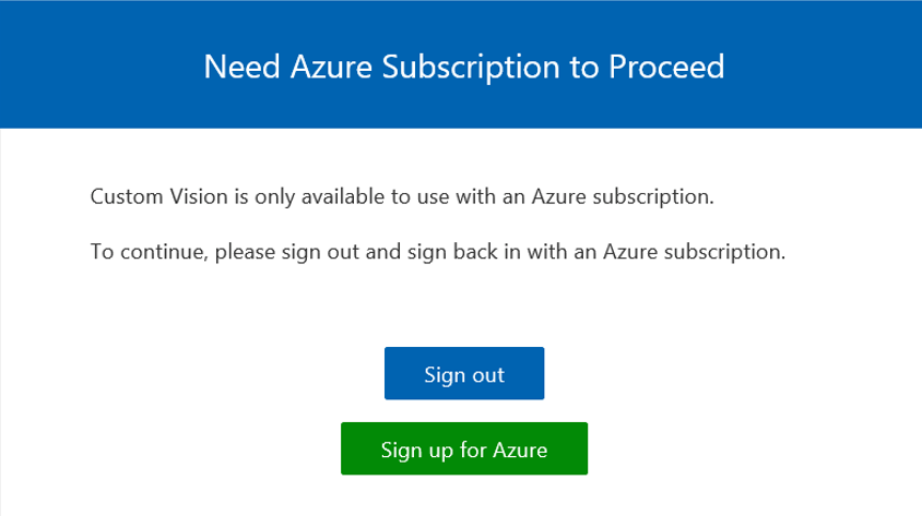
If there isn’t an Azure subscription attached to the Microsoft account you are using, you’ll see a dialog like the one shown here. Click ‘sign up for azure’ and follow the steps to create your azure account.
You should see something like the image shown here. Great! You got all of the account creation housekeeping out of the way, now on to the fun stuff!
Step 2: Collect a bunch of images showing solar panels
In this step, we’ll collect images pulled from the Vexcel image library that feature homes with solar panels on the roof. These images will be used in step 3 to train the AI model.
TIP: You need a minimum of 15 images to get started. More images will yield better results, but you can start with 15 and add more later if you like. As you collect them, try to pull a sample from different geographic regions. Rooftops in Phoenix are very different than those in Boston; try to provide diversity in your source images to ensure that the resulting model will work well in different regions.
Create a folder on your local PC to save these images too. There are several ways you can create your images of rooftops with Solar panels. One easy way is to use the GIC web application, browse the library looking for solar panels, then take a screen grab and save it to your new folder.
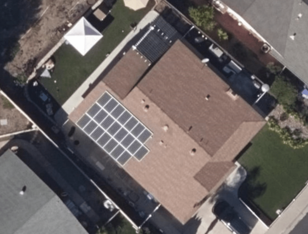
Here is an address to try this on: 11380 Florindo Rd, San Diego, CA 92127
Use a screen clipping tool to grab an image and save it to your folder. It should look something like this:
When you have 15 or more good examples of rooftops with solar panels in your folder, move on to the next step. Its time to tag our images!
Step 3: Create a new project in your Custom vision account
Click the ‘New project’ button and fill in the form like this:
For Resource, hit the ‘Create new’ link.
Your ‘New project’ form will ultimately look something like this:
Hit the ‘Create project’ button to complete the creation process. You now have a new empty project. In the next step we’ll import the images we created previously and tag them.
Step 4: Upload and Tag these images.
Your new empty project should look something like this:
Hit the ‘Add Images’ button and import all of the images you saved earlier. You should see all of your untagged images in the interface like this:
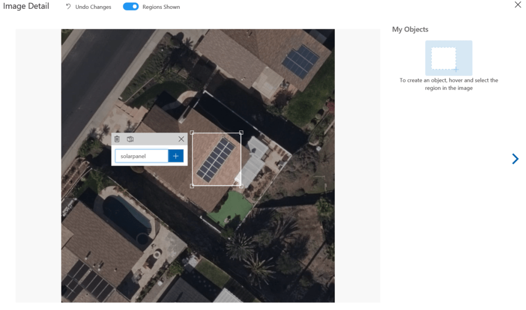
Click on the first one to begin the tagging process. Drag a box around the area of the image with solar panels, enter a new tag name of ‘solarpanel’ and hit enter.
You’ve tagged your first solar panel! Continue tagging each of the remaining images, one at a time until you have no untagged images remaining.
Step 5: Train the model
If you click the ‘tagged’ button as highlighted below, you will see all the images you have tagged. You can click on any of them to edit the tags if needed. But if you are happy with your tags, its time to train your model!
Hit the ‘Train’ button and select ‘quick training’ as your training type. Hit the ‘Train’ button to then kick off the training process. This will take around 5 minutes to complete, depending on how many images you have tagged.
Step 6: Test the model
When training completes, your screen will look something like this:
Its time to test your model! The easiest way to do so is with the ‘quick test’ button as highlighted above. Using one of the techniques used in step 2 to gather your images, go and grab a couple more and save them to the same folder. Grab some images of rooftops with solar panels of course, but also save a few that don’t have panels on the roof.
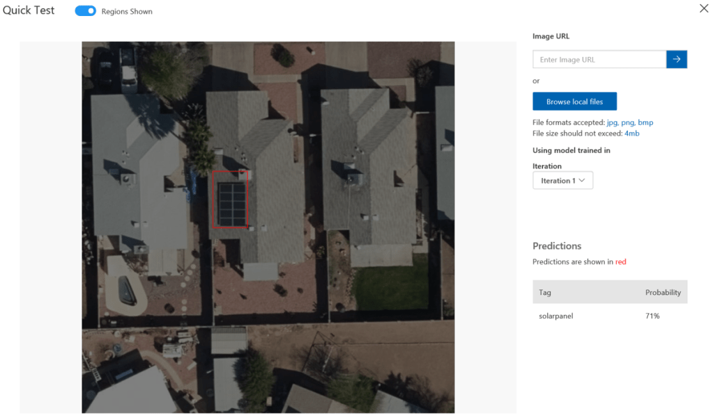
Hit the ‘Quick test’ link, and browse to select one of your new images.
As you can see here, the new model identified the correct location of the solar panels with a 71% confidence. Adding more images and running the training again will improve this. and you can go back to step 4 and do this anytime.
very cool! you just taught a machine how to identify solar panels on a roof. You can not only tag more solar panels, but you can add new tags for other entities you want to recognize in aerial imagery… Pools, trampolines, tennis courts…
In Part 2 of this tutorial series, we’ll use the same technique to operate on our disaster response imagery to identify differing levels of damage after wind events. I’ll add a link here as soon as Part 2 is online.
In Part 3, we’ll start to access the model’s we trained using the REST Api. But if you’d like to get a headstart on that and try the API out, here is a good tutorial on the custom vision website. You’ll find all of the access details you need to integrate in your app on the ‘Prediction URL’ dialog on the performance tab:
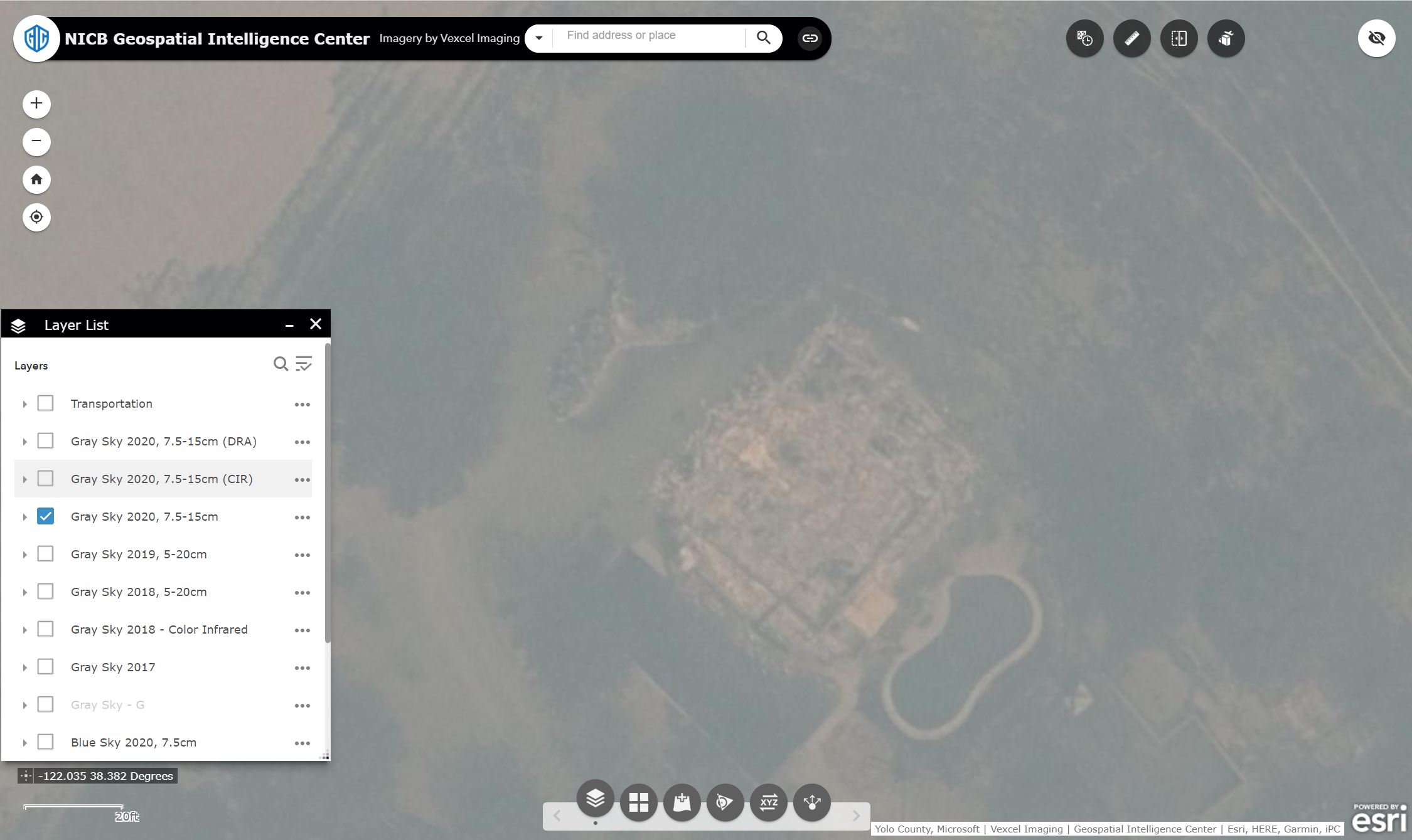
We collected and published thousands of square kilometers of imagery over the California wildfires last week. As is often the case with wildfire imagery, some areas were still in heavy smoke cover when we flew. But because we collect in the near-infrared (NIR) band along with traditional RGB, there is still a great deal of utility in the imagery for understanding damage to structures in the affected areas. Further, with some dynamic range processing, it is also possible to see a lot of detail that would otherwise be lost in the smoke. Both of these image types are available as distinct layers in our Esri based web viewer.
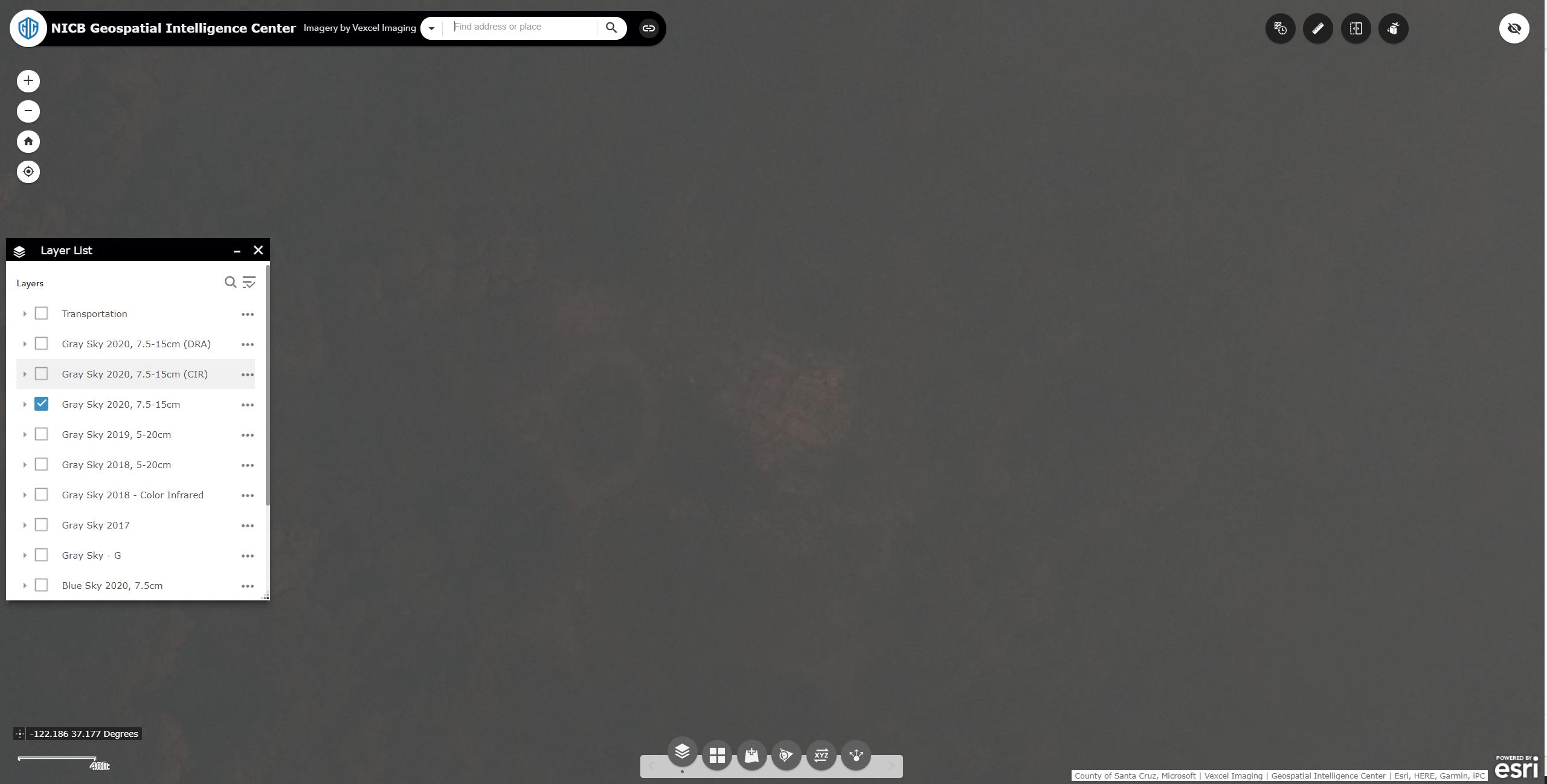
The image featured at the top of this post is an example of NIR imagery providing a good amount of detail for a property that would otherwise be nearly completely occluded with smoke. The same property is shown here in its original state, side by side with the version after dynamic range processing.
Here is another example with a heavier layer of smoke, along with the same near-infrared image. Although the NiR image may not look like a traditional RGB image you are used to, the information gleaned from it can help first responders make faster, more informed decisions in planning and logistics.
High res ortho imagery in the wake of Hurricane Laura is available for the Lake Charles region, among other areas hit hard by the storm. In this post we’ll look at the tools available in the GIC web application for Insurers to analyze their PIF or other point data sets.
The features of the viewer that we’ll focus on are:
Start by going into the viewer and searching for Lake Charles, LA. Zoom out to get an overview of the area with just the gray sky layer turned on as shown here
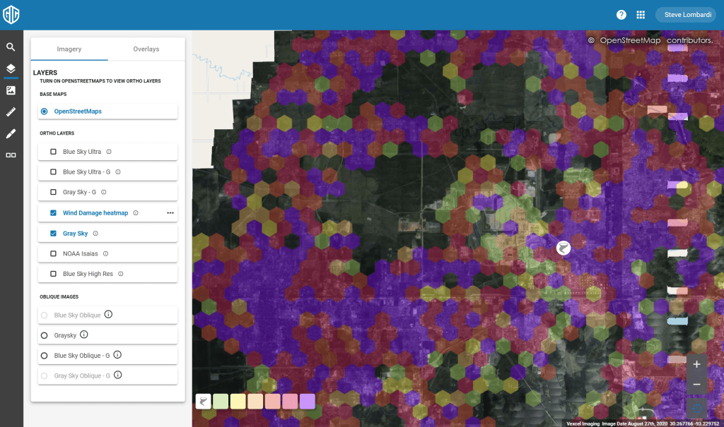
Next turn on the wind damage heatmap in the layer control. This layer is created by our partners at Munich Re using computer vision to analyze all properties in the affected region. This is a simple and very effective tool for understanding where damage in the region is greatest. As you can see here, there are almost no parts of lake Charles without at least moderate damage. The color ramp goes from light green through red and then violet indicating increasing levels of damage. Zoom in on an area and note how the hexagons ‘unfold’ to reveal more detail as you go, turning off at street level to clearly show the imagery. You can of course toggle the layer on/off at any time as well.
The Lake Charles area is approximately 900 square kilometers, far more than you could manually inspect for damage hotspots so the heatmap overlay is a very helpful tool to draw your attention to the areas of imagery with significant damage.
Next we’ll look at the data import functionality in the application. This feature is still in ‘preview’ with some added capabilities on the way, but even in the preview stage, it brings important analysis capabilities to your toolbox. You can import a variety of file formats including .KML and .SHP files, but for this tutorial we’ll use the common comma separated values (CSV) file that can be exported from Excel or any database tool. Your CSV file should contain fields for Latitude and Longitude in the first two columns, and any additional fields after that. The values in columns 3 and 4 are also important as they will be used as labels in the app.
The first line of your CSV should contain names for your fields. Latitude and Longitude should be labeled as shown, while the remainder of the labels can be whatever you like. Here is a sample that you can use:
Latitude, Longitude, AccountID, Name, notes 30.2309725, -93.3423869, P005IGPBW, Joe Smith, Your Note here 30.230995, -93.35050667, P005IGSFK, Mary Johnson, Another note here 30.233688, -93.343199, P005IGP80, Stan Lee, property note here.
Go ahead and get your CSV file setup, then come back and we’ll continue. You can save the 4 lines above in a text file on your local storage for a quick CSV file.
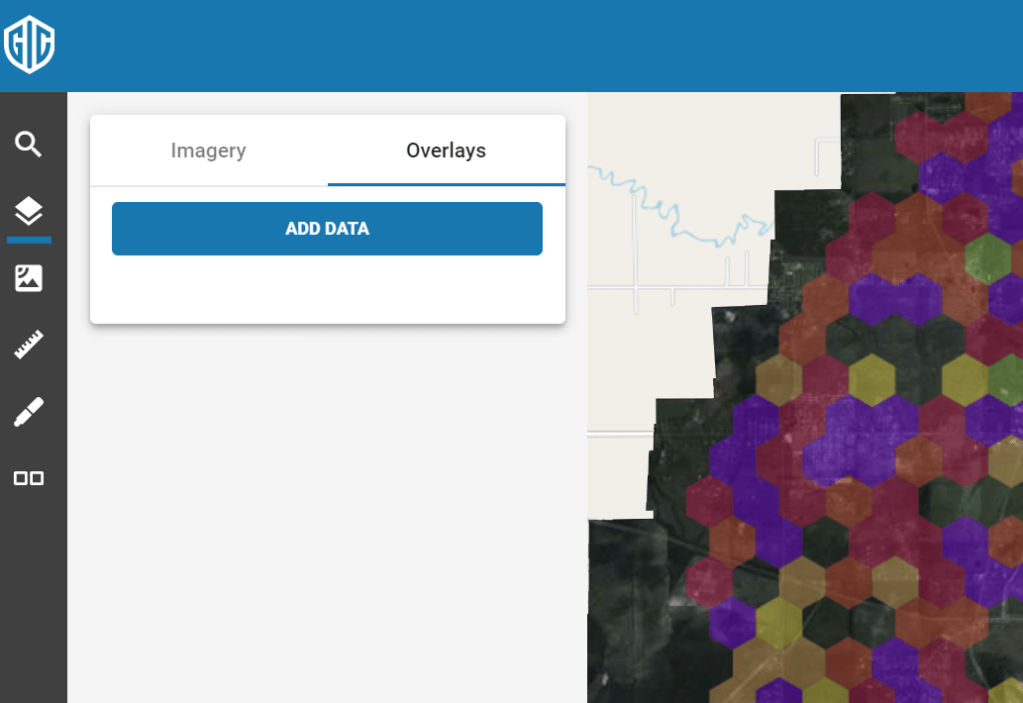
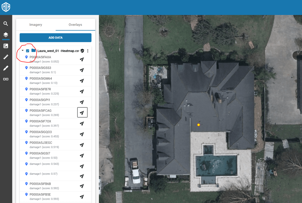
Importing is easy. Go to the Layer control in the left menu. At the top you will see two tabs; one for the imagery layers, and one for your own ‘overlays’. Choose the Overlays tab and hit the ‘Add Data’ button.
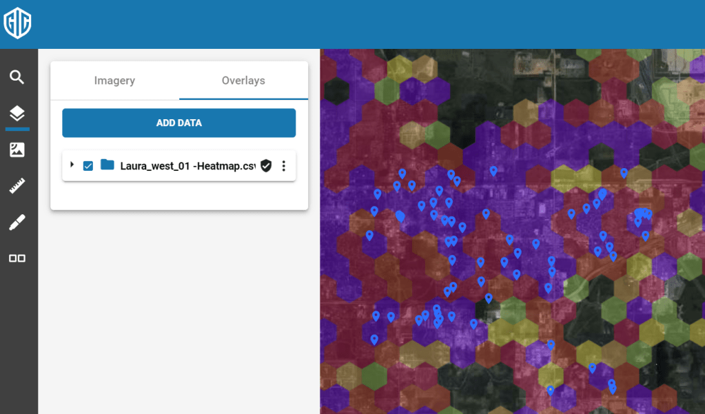
You can either browse to select your CSV file or drop it into the dialog. Either way your data is now added to the map as an overlay appearing as blue pushpins. You can toggle your layer on and off with the checkbox like any other layer.
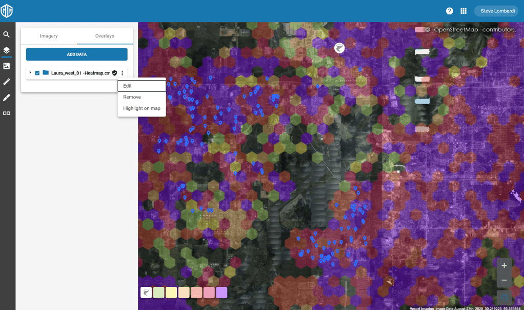
You can zoom out to see all of your points or use the ‘Highlight on map’ option on your overlay to automatically zoom out to a view that fits all of your points. You’ll find this menu choice on the … menu for your overlay as shown here:
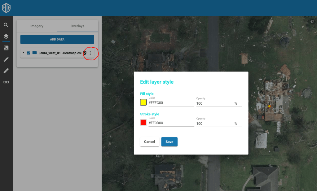
You can change the style of your pushpins with the ‘Edit’ menu choice, also found in the … menu. Here I’ve gone with a yellow pin to really pop against the imagery
And finally, you can expand your overlay to see the individual points, labeled with fields 3 and 4 from your input file. Click the icon next to any of them to center and zoom the map on that point as shown here:
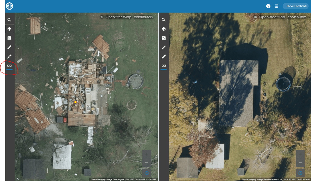
The viewer’s ‘Dual view’ feature is most often used for analysis when viewing catastrophe response imagery like our Hurricane Laura coverage. Turn it on by clicking the Dual view icon circled in the screen below. this will split the screen and provide separate layer controls for each side. In this image I have turned on the ‘Blue Sky Ultra-G’ layer with imagery from 2018. We also have 20cm imagery from 2019 in the ‘Blue sky High Res’ layer.
If you have any question on these features or any others, reach out to our tech support team at support@geointel.org